
Home |
DynOmics 1.0 |
Tutorials |
Theory |
References |
iGNM 2.0 |
Mol. Sizer&Timer |
ANM 2.0 |
Comp. Biol. Lab |
PITT site
|
|
|
Home |
DynOmics 1.0 |
Tutorials |
Theory |
References |
iGNM 2.0 |
Mol. Sizer&Timer |
ANM 2.0 |
Comp. Biol. Lab |
PITT site
|
Tutorial for DynOmics: Using Elastic Network Models – ENM 1.0
The DynOmics Portal provides information on the equilibrium dynamics of biomolecular systems using as input structural data uploaded by users. At the core of DynOmics Portal are two elastic network models: the Gaussian Network Model (GNM) and the Anisotropic Network Model (ANM). Distinctive functionalities of DynOmics Portal compared to iGNM 2.0 and ANM 2.0 interfaces include: evaluation of the (change in) dynamics in the presence of an environment (e.g. effect of multimerization or complex formation, and membrane remodeling), estimation of key sites involved in collective mechanics and allostery, and mapping of the coarse-grained conformations driven by collective modes to their full-atomic representations. See Theory for the underlying theory and assumptions.
Workflow of ENM 1.0
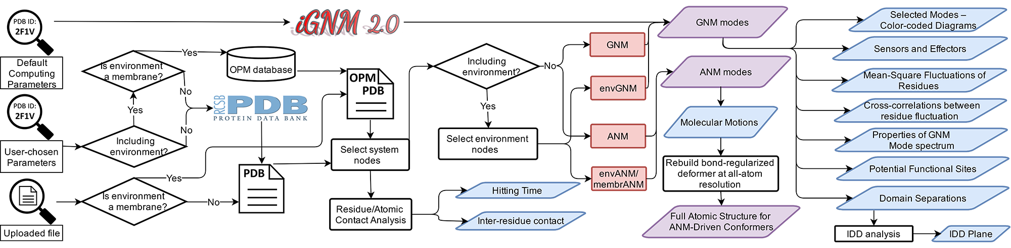
Figure. Workflow of ENM 1.0. Magnifiers on the left indicate multiple ways for users to make queries to ENM 1.0. Downloadable quantities and animated/graphed/interactive data are colored purple and blue, respectively. Calculation engines are shown in red.
1.1 Query with Default options
1.3 Considering Environmental Perturbations
Protein Dynamics
2.1 Molecular Motions – Animations
2.2 Mean-Square Fluctuations of Residues (Correlations between Experiments and Theory)
2.3 Selected Modes – Color-coded Diagrams
2.4 Residue-Residue Cross-correlations between Residue Fluctuations
2.6 Properties of GNM Mode Spectrum
Prediction for Functional Sites based on Protein Dynamics
2.8 Potential Functional Sites
2.10 Signaling/Communication Sites
1.1 Query with default options
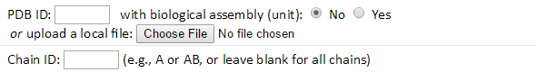
Enter the PDB (Protein Data Bank) ID (e.g., 101M) and click “Submit” button to submit a query with default options. If interested in the biological assembly (BA) structure, the “Yes” radio button should be selected. The BA structure will be downloaded from the PDB and its dynamics calculated. In addition, users may submit their own structures by clicking the “Choose File” button.
Users may also specify a chain identifier, or IDs such as AB or AC, to perform computations for only the desired chain(s).
Click “Advanced options” to expand the menu. This view may be toggled open and closed.
Closed view:
![]() Open/expanded
view:
Open/expanded
view:
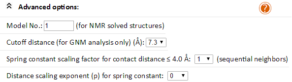
If you submit as input structural data for a Nuclear Magnetic Resonance (NMR)-solved molecule, or any input file comprised of multiple structural models/frames, you may specify the model for the calculation by choosing the Model No. of your structure.
Sophisticated Elastic Network Model (ENM) users (GNM and ANM) may also choose a desired cutoff distance to build the elastic network. The pairs of nodes with greater separation could be connected if you choose a large value. Based on our research, a broad range of cutoff distances (7-18 Å) are suitable for GNM analysis in most cases. For ANM analysis, a fixed cutoff distance of 15 Å is used.
Users may emphasize the interactions between pairs of covalently connected nodes (usually the sequential neighbor residues), by choosing a spring constant scaling factor larger than unity. Scaling factors of 10 (1) or 42 (2) have been reported to better predict the B-factors or to reproduce the low frequency spectrum derived from NMA using a conventional force field. To decrease the strength of interactions with increasing distance (s) between the interacting pairs of residues, users may increase the Distance scaling exponent (p) to > 1. The spring constant γ for pairs of residues will be rescaled by the relation: γ = s-p. Recommended scaling exponent is p = 2 (3).
1.3 Considering Environmental Perturbations
A main feature of DynOmics is the ability to generate information on the (change in the) conformational dynamics of molecules in the presence of “environmental effects.” The “environment” may be
· the lipid bilayer in the case of membrane proteins
· the neighboring molecules in the crystal lattice, for X-ray structures,
· the neighboring subunits in a multimeric protein,
· selected domain(s) or residue range in the input structure, specified by the user
· selected chain(s) of a complex (including protein-protein and protein-DNA/RNA complexes), or
· a ligand (or ligands) bound to a protein.
The dynamics in the presence of these environmental effects can be assessed on rigorous physically-based grounds: the size and number of the orthogonal normal modes are the same as those in unperturbed systems (in the absence of an environment), using our theories (4) that ensure efficient implementation (saving 3/4 time, assuming equal size of system and environment), low memory requirement (saving >1/2 memory) and more accurate evaluation of fluctuation spectra (evidenced by improved agreement with experimental B-factors). Environment considerations in the ANM theory have been published (2) and reviewed (4); their GNM counterpart is derived and implemented for the first time in this interface. GNM predictions that take account of crystal contacts have proven to yield more accurate B-factor predictions than conventional GNM.
Click “Considering Environment” to expand the menu. This view may be toggled open and closed.
Closed view:
![]() in the DynOmics home page,
in the DynOmics home page,
Open/expanded view:
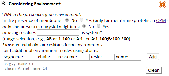
As can be seen in the above expanded view, the environment may be incorporated in three different ways: (1) membrane, (2) crystal neighbors, and (3) substrates or substructures the chain identifier and/or residue range of which is defined by the user. In all three cases, the Uploaded structures can be divided into “system and “environment.” Users assign which part of the structure forms the “system”. The rest will default to “environment.” We present below more details for submitting jobs in each case.
In case (1), users may define the membrane as environment for membrane proteins. This may be done in two ways (1) by entering a PDB code which exists in the OPM database, and (2) by generating an OPM-formatted coordinates input file (for user-uploaded structures or models). Users are asked whether their input file is OPM-formatted. They click the “Yes” option if a PDB file that is represented in the OPM database is uploaded. If not, users check the option ‘No’, which then directs them to generate an OPP-formatted coordinate file. To this aim, users are directed to the PPM server http://opm.phar.umich.edu/server.php, a sister server of the OPM database. The server evaluates the position/orientation of the user-provided membrane protein structure coordinates with respect to the membrane, and generates the PDB-coordinates file in OPM format. To use the PPM server, users should (i) upload the membrane protein user-defined coordinates onto the PPM server, (ii) click the “Submit” button to obtain the optimally positioned and reoriented protein structure, (iii) download the new coordinates using the “Download Output File” section of the PPM result page. After that, users can use OPM-formatted PDB coordinates file as input for the ENM 1.0 server to perform both envGNM and membrANM calculations. The membrane is represented as a coarse-grained (CG) ENM, the nodes and edges of which are constructed using an FCC lattice model (see Theory).
In case (2), users may define the first neighboring molecules on the crystal lattice as environment for X-ray-resolved PDB structures. The coordinates of these neighboring molecules can be evaluated using the coordinate transformation (translation and rotation) operators (required to construct molecules in adjacent unit cells) provided in the PDB files.
In case (3), the user can choose for example, the chain B for the HIV-1 protease dimeric structure (PDB code: 1A30) as the system. The protease contains two chains (chains A and B). Since chain B is treated as system, chain A becomes by default the environment. This permits to assess the effect of dimerization on the HIV-1 protease single subunit dynamics. Users may also select a range of residues as the system, e.g., you enter ‘1-100’ to select residues IDs 1 through 100 for all chains; or ‘A’ to select chain A; or ‘A:40-’ to select chain A and residue ID > 40; or ‘A:1-100;B:100-200’ to select (chain A and residue ID 1 to 100) + (chain B and residue ID100 to 200).
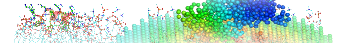
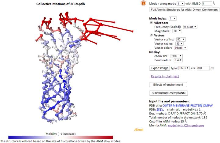
Example for including membrane as an environment (PDB ID: 2F1V):
Check the “Yes” option for “in the presence of membrane” under “Considering Environment” after entering the PDB ID 2F1V, then submit the job.
Besides, the additional environment nodes can be defined by the corresponding atom selection interface. Users are able to select any atom or any range of atoms as the additional environment nodes from the interfaces. The segment name (segname), chain identify (chain), residue name (resname), residue identify (resid) and atom name (name) can be used for the atom selection of additional environment nodes.
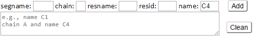
Type C4 in the name box then click Add button. Atom selection string “name C4” will be displayed as following.
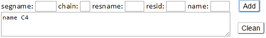
The C4 atom of residues (e.g., C4 atom of sugar residues) in the input structure will be defined as the additional environment nodes.
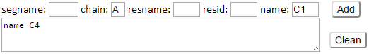
Type C1 in the name box and type A in the chain box then click Add button. Atom selection string “chain A and name C1” will be also added as the additional environment nodes.
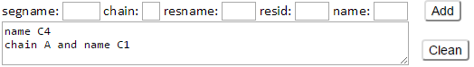
Click Clean button will remove all the added selections for the additional environment nodes.
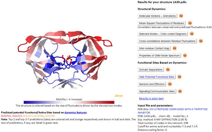
This page contains on the left, a JSmol diagram window, and on the right, Results and information on the Input file and parameters.
The JSmol window displays the PDB structure, color-coded by the size of motions driven by the lowest frequency (slowest) two GNM modes (blue: almost rigid; and red: highly mobile), as indicated by the color bar under the diagram window). We will use HIV-1 Protease (PDB id: 1A30) as an example. The corresponding Results panel and Input file and parameters are displayed below.
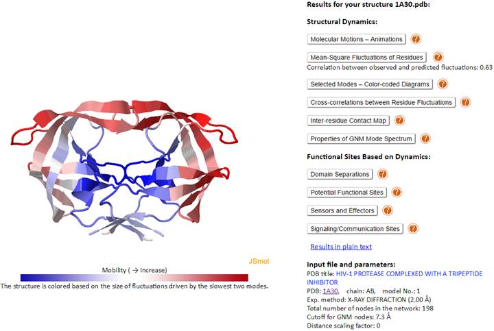
The Results panel contains ten clickable items (written below in dark blue):
Structural Dynamics
Molecular Motions – Animations
Mean-Square Fluctuations of Residues
Correlation between observed and predicted fluctuations: 0.63
Selected Modes – Color-coded Diagrams
Cross-correlations between Residue Fluctuations
Inter-residue Contact Map
Properties of GNM Mode Spectrum
Functional Sites Based on Dynamics
Domain Separations
Potential Functional Sites
Sensors and Effectors
Signaling/Communication Sites
Input file and parameters contains the input PDB ID and parameters used for DynOmics calculations. For example, the HIV-1 Protease (PDB id: 1A30) was resolved by X-ray crystallography at a resolution of 2.0 Å (Exp. method: X-RAY DIFFRACTION (2.00 Å)). Note that the Cα-atom is selected as the (single) node for each amino acid. Cutoff distance of 7.3Å (or 15 Å) is adopted for amino acid pairs in GNM (or ANM) analyses, as well as nucleotide pairs (each nucleotide being represented by three nodes; see (5)) and for mixed pairs composed of an amino acid and a nucleotide node; the spring constant for all connections is taken as unity (i.e., 1 kcal/[mol.Å2]). If the membrane environment is considered (for a membrane protein in the OPM database), a link to “model with CG membrane” will appear in at the end of the input and parameters list, which will allow for viewing the structure embedded in the modeled CG-membrane, as used in MembrANM.
2.1. Molecular Motions – Animations
This interface serves two purposes. One is to provide ANM results in the presence or absence of environment, and the second is to map a coarse-grained (CG-) model into its full-atomic counterpart, thus increasing its chemical realism (see note below) and bridging across resolutions of models. The latter, bridging scales, is done by reconstructing all-atom conformations from CG-models that are generated upon moving the structure along one of the slowest 20 ANM modes. Users may choose the size of the deformation along the selected mode by giving a root mean square deviation (RMSD) value in Å, with respect to the original structure.
Increased chemical realism entails, in addition to evaluating atomic coordinates, correcting for the over-stretched Ca-Ca pseudo-bonds. The equilibrium distance between neighboring Ca atoms is ~3.8 Å because of the coplanar nature of the three consecutive bonds - the peptide bond and the two bonds flanking the peptide bond on both sides. However, in the highly flexible regions, especially the floppy loops or parts of the N- or C-termini, the ANM-driven conformers may exhibit Ca-Ca distances larger than the standard pseudo-bond length. For such cases, here we first convert the conformers into their internal coordinates; namely, the neighboring bond length, bond angle, and dihedral angles. We maintain the bond angles and dihedral angles but readjust over-stretched or compressed neighboring Ca bond lengths back to their equilibrated length.
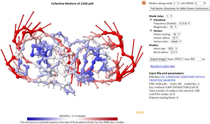
Clicking “Generate ANM deformed structures” with input of mode index and deformation RMSD, system will output reconstructed fine-grained structures based on the coarse-grained structure and motions.
envANM and membrANM
The effect of the membrane environment can be incorporated in the ANM analysis by adopting one of the following two models/methods, broadly referred to membrANM approaches:
(1) envANM-membrANM. Here the membrane is considered as the environment and the membrane protein is the system. The theory that holds for system-environment treatment is directly applicable (2). The result is the ANM dynamics of the membrane protein altered by the presence of the surrounding membrane.
(2) Substructure-membrANM. In this case, the computations are performed for the entire system, composed of membrane protein and membrane, and only the portion of the results (e.g. eigenvectors, covariance matrix) corresponding to the membrane protein is reported.
In either approach, the construction of the membrane follows the same methodology, described in the Theory, which can be found under the membrANM menu. ENM 1.0 by default reports results from envANM, as an efficient approach. Likewise, GNM results for membrane proteins in the presence of the lipid bilayer are evaluated using envGNM. Users interested in viewing the results for substructure-membrANM (which requires the decomposition of the large Hessian comprised of both membrane and membrane protein) may do so upon clicking the Substructure membrANM button above the Input file and Parameters on the right of the output page. Substructure-membrANM permits to view the motions of the membrane protein as well as those of the membrane where the protein is embedded, thus letting viewers gain insights into the coupled movements of membrane and protein.
The Substructure-membrANM is applied for membrane environment only.
Example for including membrane as an environment (PDB ID: 2F1V):
In the envANM result page, the correlation cosine (overlap) between the ANM modes predicted with and w/o environment are displayed (under the JSmol window). The correlation cosine map may be viewed by clicking the “Effects of environment” button. Note that the map will not be displayed until the completion of the calculation of the correlation cosine map.
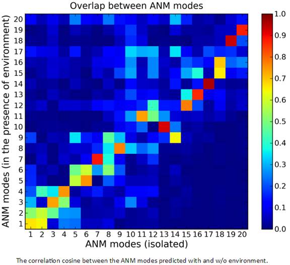
In results of envANM, the reported modes for system are full normal modes (the environment nodes are not part of the modes) which have same dimension as the normal ANM modes, see in Theory. While both the nodes of system (membrane protein) and environment (CG-membrane nodes) are parts of the normal modes with 3N + 3M dimensions (N and M are the number of nodes of system and environment respectively) in the Substructure-membrANM. Only the system part in the modes are taken and reported. Users are able to calculate and/or view the results of sub-structure MembrANM by clicking the “Substructure membrANM” button. A corresponding “envANM-membrANM” button can be clicked to go back to the envANM results page in the Substructure-membrANM results page.
The ANM modes for "Substructure-membrANM" along the ordinate of this map refer to the full spectrum of modes for the membrane protein- membrane complex. As such several low frequency modes may refer to the movements of the membrane alone, with minimal rearrangements in the protein. Note that the top 20 modes accessible to the complex account for approximately 5 of the lowest frequency modes accessible to the isolated protein in this example, consistent with the fact that the number of modes increased by about one order of magnitude upon representation of the membrane by an elastic network.
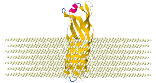
The structure of membrane protein embedded in the modeled CG-membrane can be viewed in a JSmol window by clicking the “model with CG-membrane” link. Users are able to apply colors by “Chain”, “Structure” or “B-factors” for the embedded protein.
Example of mode shapes for envGNM
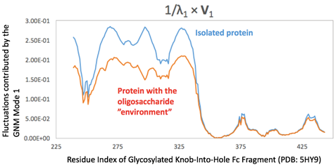
Figure. Mean square fluctuations contributed by the first GNM mode in the presence (orange) and absence (blue) of the oligosaccharide environment. The C4 atoms in the sugars are chosen as the representative nodes in the oligosaccharide complexed with disulfide-linked knob-into-hole Fc fragment (PDB ID: 5HY9; only chain B is present here, while chain A holds a similar profile). The eigenvalues and eigenvectors are obtained from the ENM 1.0 website (plain text results).
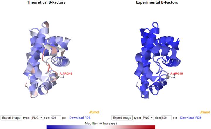
2.2. Mean-Square Fluctuations of Residues
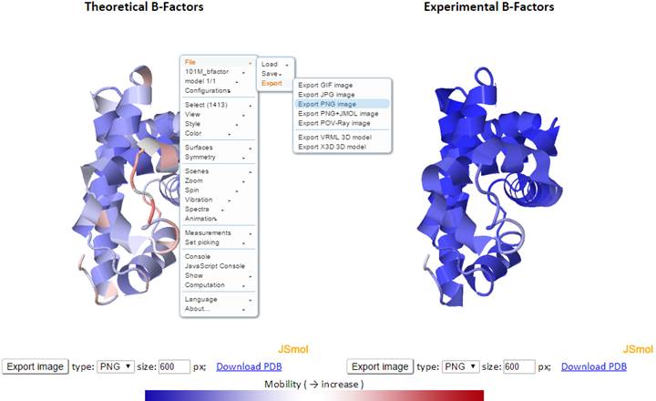
Here, the theoretical and experimental B-factors are displayed/compared using two 3D color-coded diagrams (PDB structures displayed in JSmol) and two corresponding 2D interactive graphs. Corresponding PDB structure (PDB ID: 101M), color-coded by residue fluctuations (see below), may be downloaded from the “Download PDB” link.
In the 3D JSmol window, the structures are modeled as cartoon and color-coded by GNM-defined theoretical fluctuations (left) or X-ray experimental B-factors (right) (B-factor column found in PDB files). The colors are defined by the mobility of the residues/nodes. Rigid residues are blue, and mobile residues are red.

Click “Export image” to export images from the 3D JSmol windows as different image types (PNG, JPG and GIF) and resolution (default is 600 x 600 pixels). The pop-up export dialog box for JSmol displays as
More functions may be found in the pop-up JSmol menu, viewable with a right click of the JSmol windows:
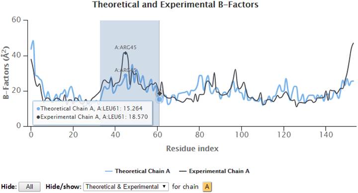
The 2D profiles of B-factors as a function of residue index are plotted using the interactive graph. The x- and y-axes refer to the residue index (ID) and B-factors respectively.
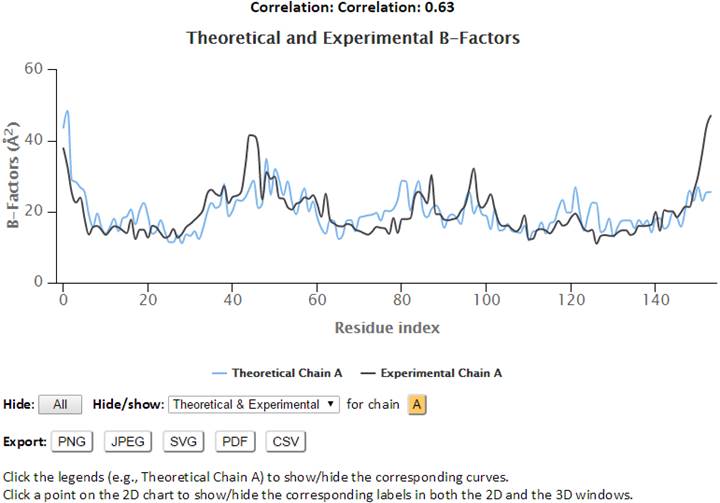
The control panel below the graph may be used to hide/show the specified chain(s) and curves (theoretical and/or experimental). Also, the experimental chains in the legend may be clicked to hide/show the corresponding plots curves on the chart. Three image formats (PNG, JPG and SVG) and/or a PDF document of the customized 2D curves may be exported by clicking the appropriate “Export” buttons. Text data in CSV format may be exported using the “CSV” Export button.
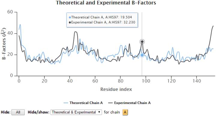
Hovering the cursor over the plots will display the plotted series with names, residues information (chain identifier, residue type and residue ID) and corresponding B-factors.
Additionally, points on the 2D plots may be clicked to label the corresponding residue in the 3D JSmol window, where Cα-atoms are represented as gray spheres, and sidechain atoms are in wireframe.
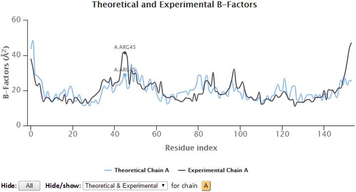
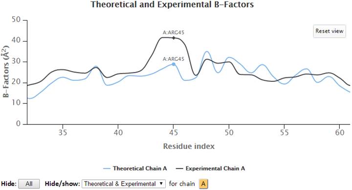
Select (click and drag) a range of the graph to zoom in to that range. A “Reset view” button appears in the top-right corner to restore the view to the molecule’s full length.
2.3. Selected Modes – Color-coded Diagrams
Similar to the B-factors results page, 3D JSmol windows and 2D interactive graphs are provided to display slow modes, fast modes, and modes averages.
The 3D structure shown in the JSmol window is color-coded based on the mobility of the residues in a particular mode. The color spectrum varies from blue (most rigid), to white, to red (most mobile).
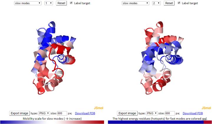
The mode types (individual slow modes, average of the slowest 1-2, 1-3 or 1-10, fast modes, and average of the fast 1-10) may be selected from the drop-down menu. Mode index (to the right of the mode type dropdown) may be selected only for the slow and fast modes, not for the averages. The default mode is slow mode, since slow modes make the largest contribution to the fluctuation of the structure and usually correlate with biological function. The coded color of the structure is updated automatically as mode type or mode index changes. Two 3D windows are provided for simultaneous visualization of pairs of modes.
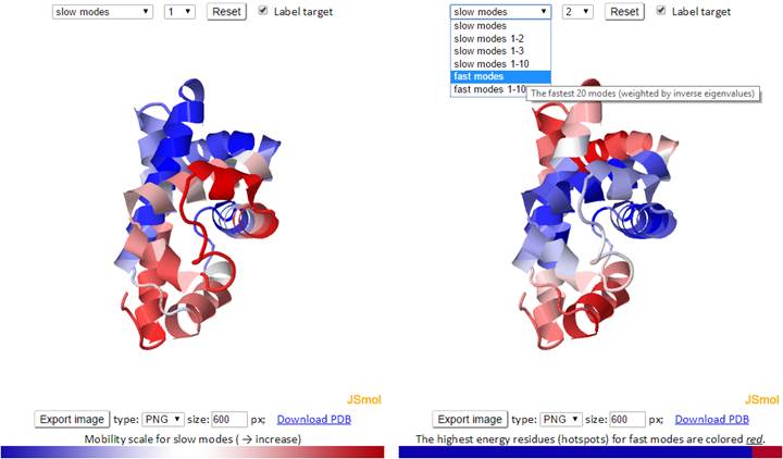
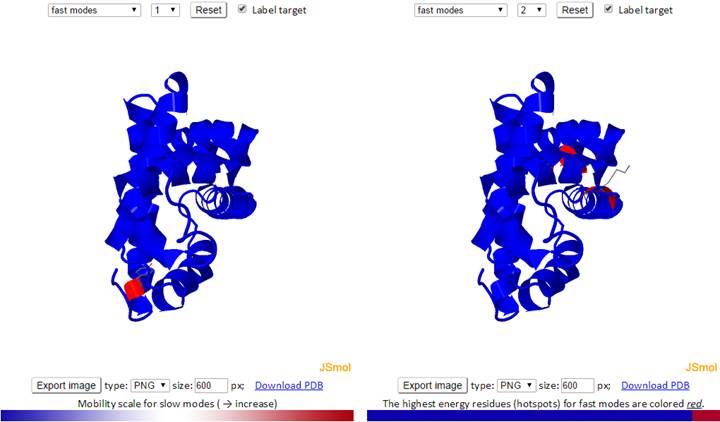
For fast modes, the whole structure is colored blue, except for hot spot residues (those subjected to highest frequency fluctuations), which are red.
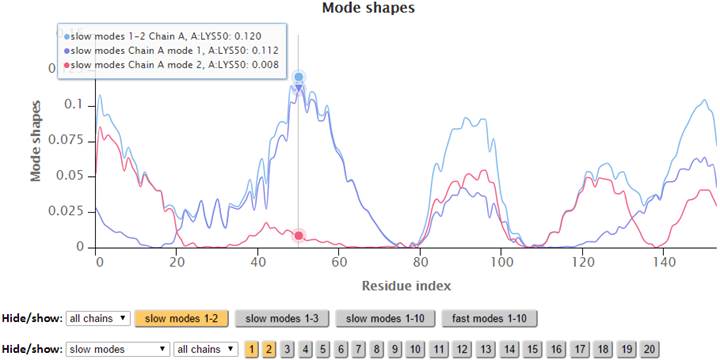
The modes in the 2D plots are scaled by the inverse eigenvalues of the Kirchhoff matrix (G). Similar to the B-factors results page, point labels and zoom-in functionality are available for the interactive 2D chart. The Hide: “All” button easily resets the chart by clearing all the plots on the chart.
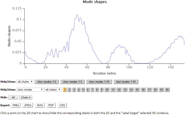
The “Export” buttons provide options to export customized figures or data in different formats. Activated buttons are highlighted orange, while inactive buttons are gray.
2.4. Cross-correlations between Residue Fluctuations
The Cross-Correlation (CC) map shows all modes by default. For PDB structures with less than 1000 nodes, the CC map may be customized with any range of modes. A customized CC map may be obtained by changing the range of modes, then clicking “Calculate.” Residue numbers (i,j) along the axes refer to those of all chains, ordered by chain index.
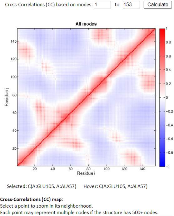
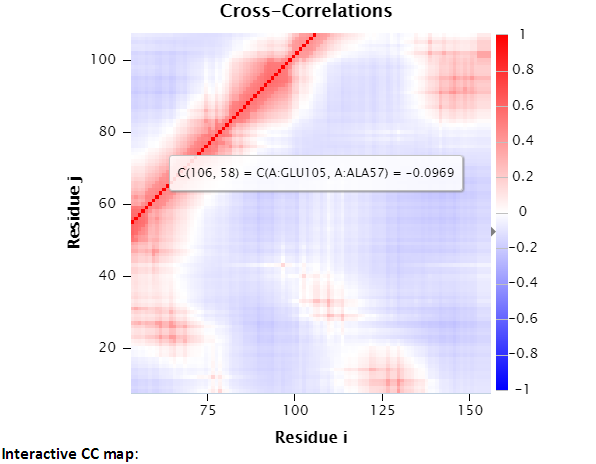
Two CC maps (static on the left, interactive on the right) are shown for those structures composed of < 1,000 nodes. As the cursor moves over the static (left) CC map, information for the pair of residues of interest is displayed below the map. By clicking a point on the static map, the interactive (right) CC map will display a zoomed in view containing 100 residues on both axes, centered at the selected point on the static map. The interactive CC map allows even large structures to be displayed clearly.
An example of an interactive CC map of PDB ID: 101M in action, when a point (A:GLU105, A:ALA57) is selected on the static CC map:
The size of interactive CC map may be customized using the control panel below the map. The minimum residue indices i and j can be changed, as well as the map size. The maximal indices are automatically calculated based on the minimal index and the map size (e.g., there are 100 points between min i 45 and max i 144). “Redraw” redraws the interactive CC map based on the settings (min i, j and the map size which defines the map range) in the control panel. The following interactive CC map will be drawn using settings: map size = 100, min i = 45, and min j = 6.
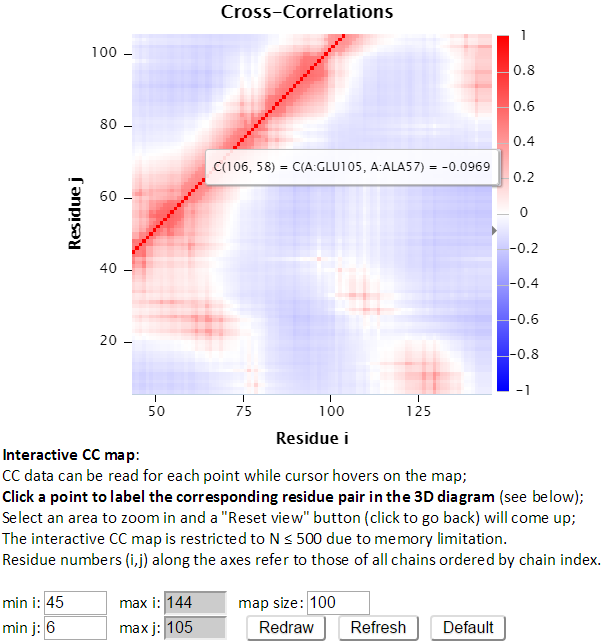
“Refresh” not only redraws the interactive CC map using the settings, but also reloads the page with a new URL address with the new settings. For example, http://gnmdb.csb.pitt.edu/iGNM_CC_map.php?gnm_id=101M&modes=cc_all&x_min=45&x_max=144&axis_length=100&y_min=6&y_max=105&max_length=800 is the URL of the page generated by clicking “Refresh” with the above settings selected. The URL directly restores the customized settings and view of the above interactive CC map, therefore it can be saved/shared for later viewing. “Default” resets the settings to the defaults.
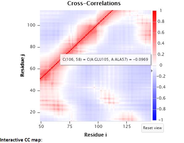
The interactive CC map can be magnified by selecting a range of points on the map. “Reset view” will reset the interactive CC map back to the original view.
Selecting a point (e.g., A:GLU105, A:ALA57) on the interactive CC map will label the Cα-atoms of the pair of residues (shown as spheres, and of the same color as the selected point) in the 3D JSmol window.

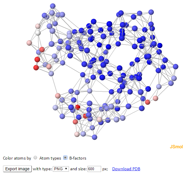
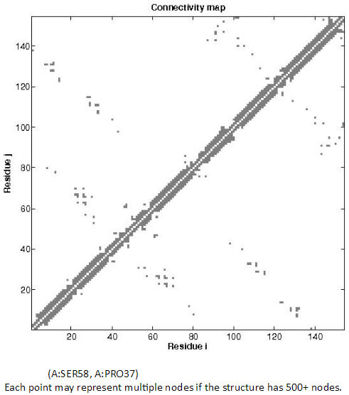
2.5. Inter-residue Contact Map
The GNM representing the structure is displayed (spring-and-bead representation) on the left, and the corresponding 2D inter-residue connectivity/contact map is shown on the right. Each sphere represents a node, and each line between the nodes represents a spring connection/interaction between the pair of interest. Nodes are connected if they are located within the cutoff distance.
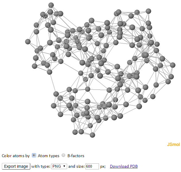
The color of atoms/nodes (spheres) can be changed by clicking the radio buttons “Atom types” and “B-factors.” Like the 3D B-factors windows, images can be exported using “Export image” button.
The topology of the network can be viewed in the 2D Connectivity map. Each dot represents a spring connection between residue i and j. Residues IDs can be seen by hovering over of the points of interest on the CC map.
2.6. Properties of GNM Mode Spectrum
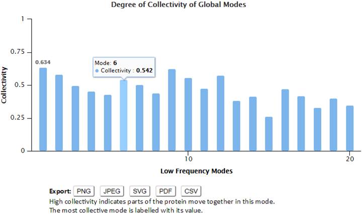
The motion frequency of GNM modes have been evaluated by 1/λ (reciprocal of eigenvalue). A higher value indicates a slower mode with low frequency. The low frequency modes are highly relative to the biological functions.
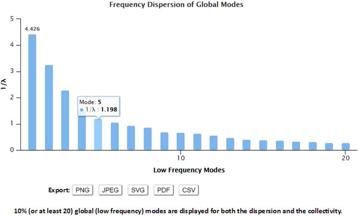
The degree of collectivity of a given mode measures the extent to which the structural elements move together in that particular mode. A high degree of collectivity means a highly cooperative mode that engages a large portion of (if not the entire) structure. Conversely, low collectivity refers to modes that affect small/local regions only. Modes of a high degree of collectivity are generally of interest as functionally relevant modes. Such modes are usually found at the low frequency end of the mode spectrum. The degree of collectivity of these low frequency modes is shown in a bar plot (below). Hovering the cursor over the bar of each mode will display the mode number and its corresponding degree of collectivity. Users may select and enlarge a range of modes in the bar plot, and the figure and data can be exported in different formats using the Export buttons.
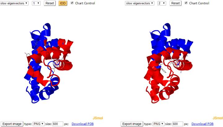
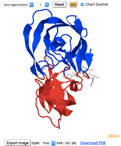
Blocks of residues are divided into separate domains based on the direction (+/-) of their movement in the slowest modes. To this aim, we examine the sign (+/-) of the elements (residues) in the selected mode eigenvector. Residues with the same sign move together in the same direction, and are therefore assumed to form a dynamically coupled domain, also called intrinsic dynamic domains (IDDs). The interfacial residues are shown using wireframe representation. The 3D JSmol windows and the 2D interactive graphs have the same functionalities as the Mode Shapes result page.
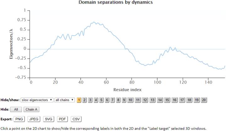
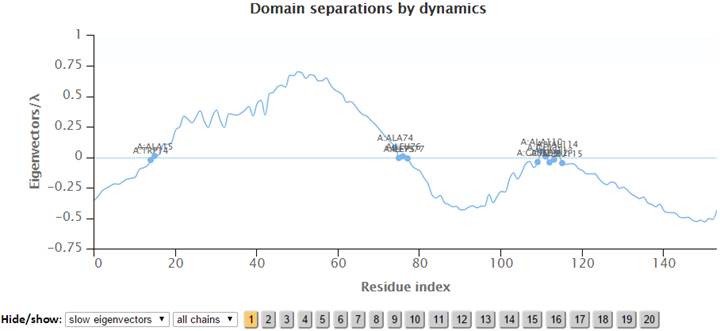
The labeled residues in the “Domain separations by dynamics” chart below are the interfacial residues whose neighboring residues have a different sign in the eigenvector relative to themselves. The interfacial residues act as hinges in the movement of the molecules.
Within the past two years, we have established the concepts of IDDs defined by the slowest normal modes, and their use to predict active sites (6), protein-protein docking poses, (6) and protein-DNA docking orientations (7). The normal modes can be derived from GNM or ANM analysis of a single structure or from the principal component analysis (PCA) of a collection of experimentally determined structures or MD snapshots.
According to our previous results (6,7), the GNM slowest modes provide the richest information suggesting functional sites or molecular interaction orientations. Hence, in DynOmics, we provide: (A) IDDs; (B) a dynamics(D-) plane that, mathematically, best divides the two largest anti-correlated domains (the (+) and the (-) domains); and (C) the domain(D-) axis projected from the axis that best outlines the distribution of the transition points for 3 slowest modes. (Note: “Transition points” indicate the inter-domain interfacial nodes that are flanked by one node from the (+) blue domain and one node from (-) red domain in the primary sequence.) For more information, click “IDD”.
The D-plane partitions the protein structure in two domains (green plane, shown in the figure below). The IDDs (in blue and red) depend on the selected GNM mode. The D-axis is displayed as a thick blue line on the D-plane.
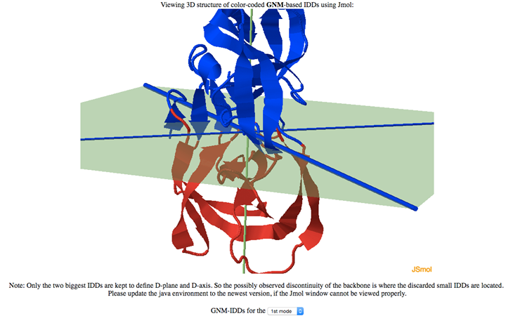
D-plane normal, D-axis vector, center of transition points, and separation quality F(n) (higher F(n) means better domain separation) are provided in the same interface, as shown below.
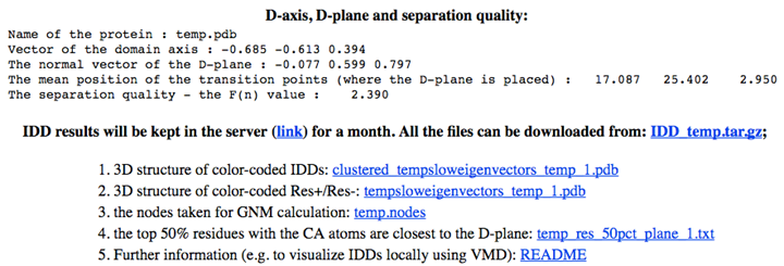
Then, how to use the results from IDD analysis? First, we have previously found that 90% of the active sites lie within 50% of the residues closest to the D-plane (6). In addition, D-planes were shown to cut through the protein’s binding partners, that is, either another protein (6) or DNA (7). Furthermore, cross angles for the D-axes of the protein binding partners were found to be > 70 degrees. Combining the statistical results for D-plane cutting and D-axes angles, it has been shown that utilizing the D-plane and D-axes angles can help enrich the rate of finding native decoys by 2.5 fold, as compared to the standard protein-protein docking method (6). Thus, IDD results help sort the most promising docking decoys from protein-protein docking poses and protein-DNA docking poses.
2.8. Potential Functional Sites
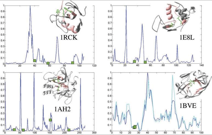
Inspired by our PCA_NEST tool (8), we use here GNM slowest two modes and the same algorithm to predict potential functional sites (PFSs). The algorithm, referred to as the minima-screening algorithm, depends on inter-residue contact topology exclusively, irrespective of residue type or evolutionary conservation. The PFSs are the hinge residues that control the slowest modes, selected and rank-ordered based on their relative solvent accessibility and spatial clustering properties (8-10). Using this algorithm, we were able to locate the majority of catalytic residues within the top-ranking 6–8 PFSs (8).
The interface in the main results page provides the 3D structure of interest. The residue identities of predicted PFSs will be listed under the diagram once users clicked the “Potential Functional Sites” button (or by clicking the same button with automatically edited name “Hide Potential Functional Sites” to hide them in the interface). The side chain of the top-ranked predicted PFSs will be displayed in red stick-and-ball (top two predictions) or orange stick-and-ball (top 3-7 predictions).
http://www.ebi.ac.uk/thornton-srv/databases/CSA/SearchResults.php?PDBID=1a30&SUBMIT_PDB=SEARCH+CSA
The catalytic sites of HIV-1 protease (PDB ID: 1A30) recorded in the Catalytic Site Atlas (CSA) database are residues A:ASP25 and B:ASP25. B:ASP25 is ranked as the top 1 predicted PFS.
Two examples of PFS predictions:
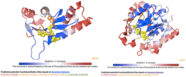
Figure. The catalytic residues in ASV integrase core domain (PDB ID: 1A5V, right) and phosphatidylinositol-specific phospholipase C from Listeria Monocytogenes (PDB ID:2PLC, left) are presented in yellow VdW spheres. Top 2 and top 3-7 potential functional sites/residues predicted by the COMPACT algorithm are shown in red and orange ball-and-stick, respectively. In these two specific cases, the average distances between catalytic residues and protein mass centers are 9.3 and 10.8 Å for ASV integrase and phospholipase C, respectively.
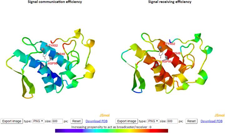
On the initial page, enter the PDB ID (e.g., 4B9Q), and type “A:4-530” in “or using residues” at “Considering Environment”. Here, we consider residues from 4 to 530 of chain A for ATP-bound DnaK. Click “Submit” button to submit a query. In the result page, click “Sensors and Effectors”. In another page, we have the results of “Sensors and Effectors”. On top panel, there are two ribbon diagrams showing sensor (left) and effector (right) residues as shown below.
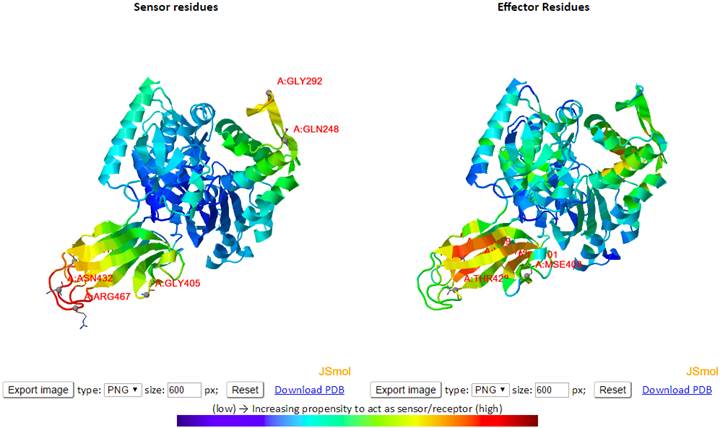 High
sensor/effector residues are shown in dark red as shown in color bar. We can
rotate structures and change their sizes using mouse. We can download the
structure with different resolutions we can choose at “size” and different file
types. Below the structures, there is a map and two graphs.
High
sensor/effector residues are shown in dark red as shown in color bar. We can
rotate structures and change their sizes using mouse. We can download the
structure with different resolutions we can choose at “size” and different file
types. Below the structures, there is a map and two graphs.
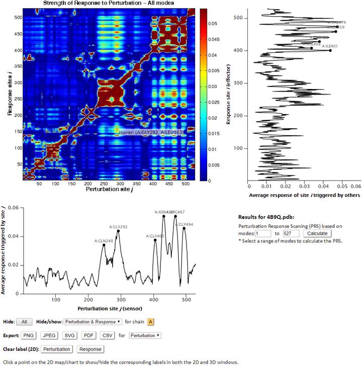
On the PRS map, strong responses are shown in dark red. The peaks along the curves indicate the residues that can potentially serve as sensors (the graph below the map) and effectors (right side of the map). In both graphs, we can zoom-in the graph and mark residues by clicking. The marked residues are also automatically shown in the structures on top. Below the sensor graph, there are three options. “Hide” is useful for a system with multiple chains. By clicking “Hide” with a chain, we can hide the chain, and by clicking the ID (A) at chain, we can show the chain again. By clicking “Export”, we can download the graph of Perturbation or Response with different image file types. By clicking Perturbation or Response at “Clear label (2D)”, we can remove labels we did. Below the effector graph, there is a section as shown below.
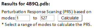
Here, we can change range of modes to calculate PRS (default is all modes).
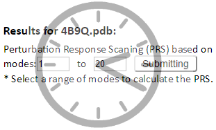
After choosing different modes and clicking “Submitting”, we have new results of map, graph, and structures calculated based on the range of modes we selected.
2.10. Signaling/Communication Sites
Hitting and commute times are graph-theoretical concepts based on Markovian processing of signals across the network (see Theory page). Two ribbon diagrams are shown on the page, which reflect the propensity of residues to send signals (left ribbon diagram, color-coded), or to receive signals (right ribbon diagram, color-coded). Smaller hitting time (as receiver or broadcaster) indicates higher propensity for (allosteric) communication. The values for individual residues in those ribbon diagrams are deduced from the 2D map shown on the same map, by taking the average of rows and columns, as indicated. The residue info (chain ID, residue name and residue ID) can be viewed on the hitting time curves profiles (along both axes) and on the map by hovering the cursor on the curves or on the map. Clicking a point on the chart will add a label to the plot as well as the corresponding residue in the 3D viewer. The chain(s) can be shown/hidden via the interactive chart control buttons. Similar to the chart function, clicking a point on the map will label the corresponding pair of residues in the 3D viewers.
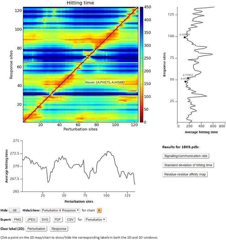
Commute time is also provided at the bottom of the same page. Based on the theory, hitting time H(i,j) is asymmetric, while the commute time C(i, j) = H(i, j) + H(j, i) is symmetric.
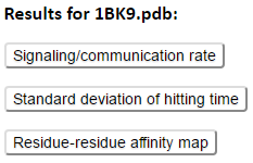
To the right of the Hitting time map, user will find three buttons to view the “Signaling/communication rate”, “Standard deviation of hitting time” and “Residue-Residue affinity map” result pages.
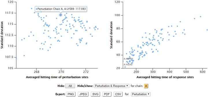
In addition to the hitting time, the server also releases the hitting rate, which is simply the ratio Rij /Hij where Rij is the distance between residues i and j in the equilibrium (resolved) structure. The results of hitting rate can be viewed in the “Signaling/communication rate” result page. The “Standard deviation of hitting time” result page displays the standard deviations vs mean value for both response sites and perturbation sites. Standard deviation refers to the variation in the hitting time of a given receiver (or sender) residue depending on the 2nd residue that serves as sender (or receiver). User can read the residue info while hovering the cursor on the points of map, and label the corresponding residues in 3D viewers by clicking the points. Overall, residues exhibiting higher average hitting times also show higher standard deviation value. Sites with low average hitting time and standard deviation are distinguished by their efficient and precise function with regard to signal transmission.
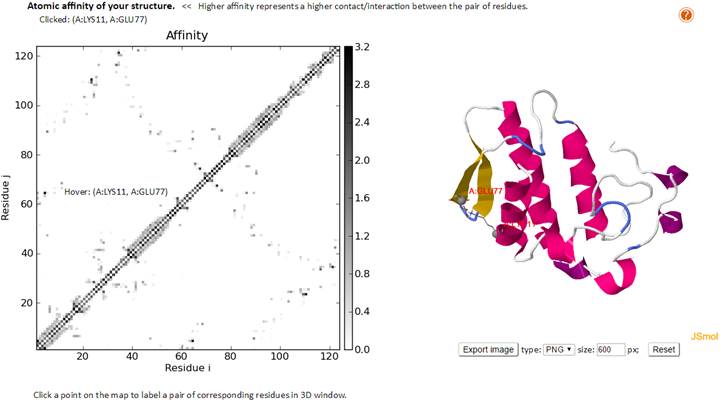
The “Residue-Residue Contact affinity map” results page reports the contact affinities for each pair of residues based on their atom-atom contacts. Hitting times are computed based on these affinity matrices (used in the Markovian stochastics model). By clicking the points which indicate the pairs of interacting residues, user can see the location of the residue pairs in the 3D structure.
The nodes files in PDB format, network topology, and GNM Kirchhoff matrix used for the GNM calculation are listed. The GNM outputs including eigenvalues, slow modes, fast modes, slow eigenvectors, fast eigenvectors, slow mode average 1-2, slow mode average 1-3 and fast mode average 1-10 are provided. The text format of cross-correlations (for structures have nodes less than 1000 only); slow modes collectivity; vibrational entropy (11); theoretical and experimental B-factors; along with the scaling factor and the estimated spring constant, are provided in the text format.
Descriptions for the plain text files
|
Filename |
Description |
|
(PDB Code)_nodes.pdb |
The GNM nodes file in PDB format. |
|
(PDB Code)_connectivity.txt |
The connectivity (topology) of model in sparse form. 3 columns, comprising two nodes indices columns and a connectivity type column (1, 2 and 3 refer to the connection between amino acid pairs, nucleotides pairs and amino acid – nucleotide pairs, respectively). |
|
(PDB Code).kdat |
The GNM Kirchhoff matrix in sparse form. |
|
(PDB Code).cont |
Lists the number of neighbors in contact with a specific residue within a cutoff of 7.3 Å |
|
(PDB Code)_resnum.txt |
Contains the number of nodes in the model. |
|
(PDB Code).bfactor |
Contains the theoretical and experimental B-factors (temperature factors). It has 5 columns. The columns 1 to 3 refer to chain identifiers, residue names and residue indices, respectively; column 4 and 5 are the GNM calculated theoretical B-factors and the x-ray crystallographic b-factors taken from the PDB file. |
|
(PDB Code)_scaling.txt |
Prefactor used to scale theoretical fluctuations to experimental B-factors. |
|
(PDB Code)_gamma.txt |
Estimated value of spring constant. |
|
(PDB Code).eigen |
Lists N eigenvalues in increasing order. 1st eigenvalue is a zero value. |
|
(PDB Code)_entropy.txt |
The GNM-defined vibrational entropy based on Karplus’ method (1981). |
|
(PDB Code).slowmodes |
23 or more (to keep 40% of the spectrum) columns. The columns 1-3 refer to chain identifiers, residue names and residue indices, respectively; columns 4-23 (or more) are slow mode shapes associated with the 20 (or more) slowest (lowest frequency) modes, starting from the slowest (first) mode. |
|
(PDB Code).slow2av |
4 columns. The columns 1-3 refer to chain identifiers, residue names and residue indices, respectively; column 4 is the residue mean-square fluctuations driven by the joint contribution of the slowest two modes. |
|
(PDB Code).slow3av |
4 columns. The columns 1-3 refer to chain identifiers, residue names and residue indices, respectively; column 4 is the residue mean-square fluctuations driven by the joint contribution of the slowest three modes. |
|
(PDB Code).slow10av |
4 columns. The columns 1-3 refer to chain identifiers, residue names and residue indices, respectively; column 4 is the residue mean-square fluctuations driven by the joint contribution of the slowest ten modes. |
|
(PDB Code).fastmodes |
23 columns. The columns 1-3 refer to chain identifiers, residue names and residue indices, respectively; columns 4-23 are fast mode shapes associated with the 20 fastest (highest frequency) modes, starting from the highest mode. Since the last modes reflect localized fast motions in the protein, these modes have only a few non-zero elements. |
|
(PDB Code).fast10av |
4 columns. The columns 1-3 refer to chain identifiers, residue names and residue indices, respectively; column 4 lists the residue mean-square fluctuations driven by 10 modes having the highest frequency. |
|
(PDB Code).sloweigenvectors |
23 columns. The columns 1-3 refer to chain identifiers, residue names and residue indices, respectively; columns 4-23 are the elements of eigenvectors associated with the 20 slowest (lowest frequency) modes, starting from the slowest (first) mode (column 4). |
|
(PDB Code).fasteigenvectors |
23 columns. The columns 1-3 refer to chain identifiers, residue names and residue indices, respectively; columns 4-23 are the elements of eigenvectors associated with the 20 fastest (highest frequency) modes, starting from the highest mode (column 4). |
|
(PDB Code)_cc_all.txt |
The file contains the cross-correlations for all modes between residue fluctuations. The values are between +1 (perfect concerted motion) and -1 (perfect anti-correlated motions). The file is provided for structures having no more than 1000 nodes only. |
|
(PDB Code) .collectivity-slow |
The file contains N/10 (where N is the nodes number) or at least 20 collectivity values of the slowest modes. |
Particularly,
the vibrational entropy (12) is calculated as
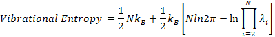
where kB is Boltzmann constant; λi is the eigenvalue of the ith mode; N is the number of nodes of the structure. For example, the GNM-defined vibrational entropy of PDB 101M is -294.07 kB.
The collectivity (13) is defined as
![]()
where, k is the mode number; N is the number of nodes of the structure; ΔRi is the displacement of the ith residue. If Collectivity = 1, the residues have equal contribution in the kth mode; if it is 1/N, it means that only one node contributes to the fluctuation.
1. Kondrashov, D.A., Van Wynsberghe, A.W., Bannen, R.M., Cui, Q. and Phillips Jr, George N. (2007) Protein Structural Variation in Computational Models and Crystallographic Data. Structure, 15, 169-177.
2. Ming, D. and Wall, M.E. (2005) Allostery in a coarse-grained model of protein dynamics. Phys. Rev. Lett., 95, 198103.
3. Yang, L., Song, G. and Jernigan, R.L. (2009) Protein elastic network models and the ranges of cooperativity. Proc. Natl. Acad. Sci. U. S. A., 106, 12347-12352.
4. Bahar, I., Lezon, T.R., Bakan, A. and Shrivastava, I.H. (2010) Normal Mode Analysis of Biomolecular Structures: Functional Mechanisms of Membrane Proteins. Chem. Rev., 110, 1463-1497.
5. Yang, L.-W., Rader, A.J., Liu, X., Jursa, C.J., Chen, S.C., Karimi, H.A. and Bahar, I. (2006) oGNM: online computation of structural dynamics using the Gaussian Network Model. Nucleic Acids Res., 34, W24-W31.
6. Li, H., Sakuraba, S., Chandrasekaran, A. and Yang, L.-W. (2014) Molecular Binding Sites Are Located Near the Interface of Intrinsic Dynamics Domains (IDDs). J. Chem. Inf. Model., 54, 2275-2285.
7. Chandrasekaran, A., Chan, J., Lim, C. and Yang, L.-W. (2016) Protein Dynamics and Contact Topology Reveal Protein–DNA Binding Orientation. J. Chem. Theory Comput., 12, 5269-5277.
8. Yang, L.W., Eyal, E., Bahar, I. and Kitao, A. (2009) Principal component analysis of native ensembles of biomolecular structures (PCA_NEST): insights into functional dynamics. Bioinformatics, 25, 606-614.
9. Bartlett, G.J., Porter, C.T., Borkakoti, N. and Thornton, J.M. (2002) Analysis of Catalytic Residues in Enzyme Active Sites. J. Mol. Biol., 324, 105-121.
10. Gutteridge, A., Bartlett, G.J. and Thornton, J.M. (2003) Using a neural network and spatial clustering to predict the location of active sites in enzymes. J. Mol. Biol., 330, 719-734.
11. Zimmermann, M.T., Leelananda, S.P., Kloczkowski, A. and Jernigan, R.L. (2012) Combining Statistical Potentials with Dynamics-Based Entropies Improves Selection from Protein Decoys and Docking Poses. J. Phys. Chem. B, 116, 6725-6731.
12. Karplus, M. and Kushick, J.N. (1981) Method for estimating the configurational entropy of macromolecules. Macromolecules, 14, 325-332.
13. Brüschweiler, R. (1995) Collective protein dynamics and nuclear spin relaxation. J Chem Phys, 102, 3396-3403.