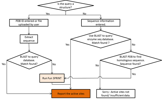
Functional Site PRIoritization NeT (FunSPRINT) gathers proteins' sequence, structure and dynamics information to predict locations of active sites or non-catalytic functional sites in enzymes or proteins with known or unknown functions. The web service features the following –

A. The web server is designed for enzymes with all spectrum of catalytic functions, not tailored for a specific enzyme class or family. The training set contains enzymes derived from all the six enzyme classes.

B. The server uses protein dynamics as an important feature. Over 240 enzymes, we found 86% of the overall 732 catalytic residues are co-localized with the dynamics hinges, the local minima of the fluctuation profile that outlines the superimposition of three slowest normal modes along the residue index. The low-frequency dynamics and their corresponding normal modes are characterized by the elastic network model (ENM; which is one of the reasons we use the word ‘net’ for the name of the server).

C. The Partial Least Square (PLS) regression model was trained not by directly taking the values in each feature but by taking the differences between catalytic and non-catalytic residues in each feature according to which all the catalytic and non-catalytic residues are ranked within an enzyme. That relative difference between catalytic and non-catalytic as well as residues’ rank in each feature are taken implies that the server predicts those residues that are most prioritized in all the features and also implies that we suggest ‘functional’ residues for any protein including those believed to have no function.

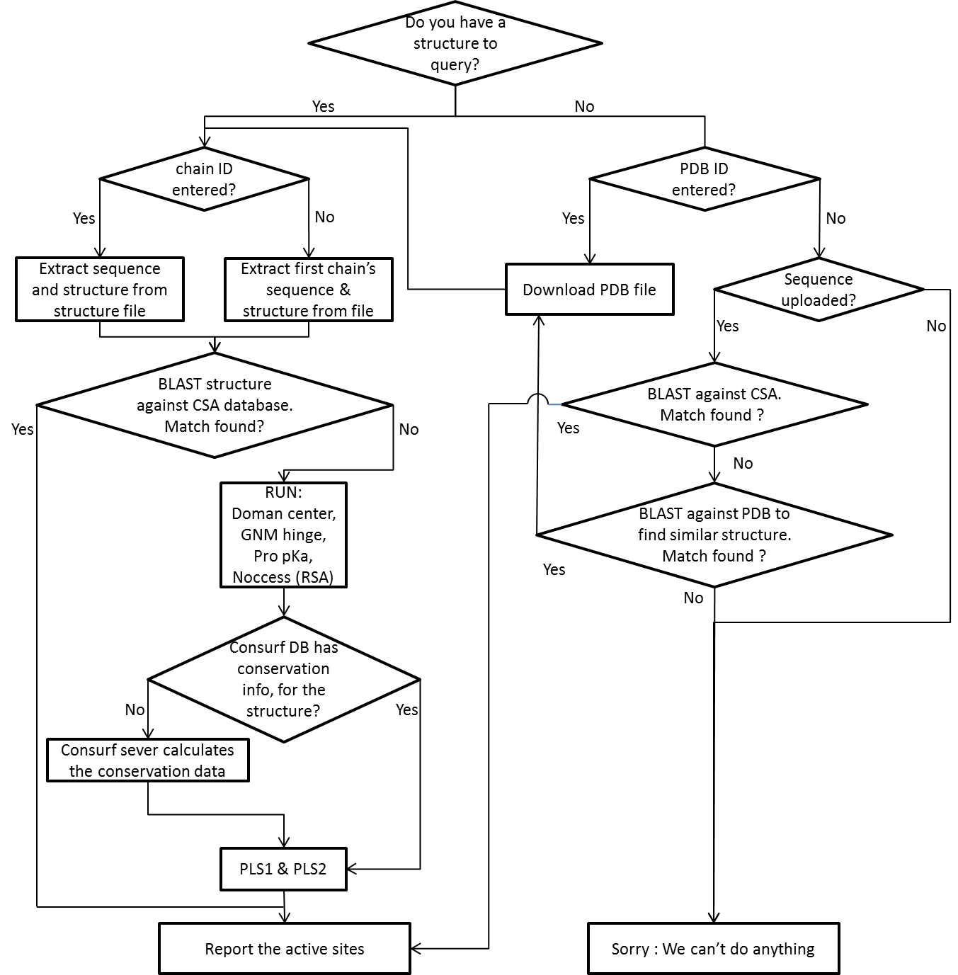
The workflow of the server is summarized below (see a detailed version)

How to use the server?

Please view the help page

Features used in the prediction models:

Two consecutive PLS regression procedures are used in the functional site prediction. The first PLS takes features including Conservation scores (sequence feature), Residue Propensity (sequence feature), pka changes (structure feature), Solvent accessibility surface area, or SASA (structure feature), Distance to mass center (structure feature), Dynamics hinges (dynamics feature) for the model building. With the prediction results from the first PLS, The second PLS takes two more features that are Weighted clustering scores (structure feature), Deviation of SASA of neighboring residues (structure feature) to make the final predictions.

Conservation scores (sequence feature)

Conservation indicates how well-preserved a residue is between species in the course of evolution. The conservation feature of active site prediction utilizes the ConSurf server (http://consurf.tau.ac.il/) to determine the level of evolutionary conservation of protein residues based on phylogenetic relationship among species (Glaser, et al., 2003).

Evolutionarily conserved residues may possess biological functions or structural significance and may thus serve as possible catalytic sites. FunSPRINT first queries ConSurf to calculate the conservation scores for the submitted PDB file (if users do not provide one by themselves), the process of which may take up to hours considering the availability of information in the ConSurf database (see the Figure below).

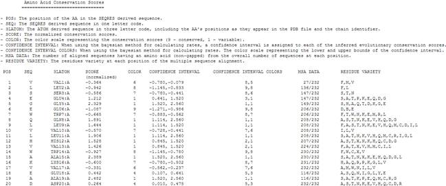
FIGURE. Example page from ConSurf showing the result of calculated conservation scores of amino acids of a given protein sequence. Users are recommended to obtain such a file from ConSurf server and then submit it to our FunSPRINT, otherwise the computation could take much longer.

The residues are then categorized into 9 levels according to the acquired conservation scores, with level 9 as the most conserved and level 1 the least conserved.

Residue Propensity (sequence feature)

The value of residue propensity is determined by the catalytic propensity proposed by Janet Thornton et al. in previous studies based on the analysis of 615 catalytic sites in 178 proteins (Bartlett, et al., 2002). Catalytic propensity is defined by dividing the ratio of a certain amino acid acting as a catalytic site to all the catalytic residues by the ratio of that particular amino acid to all the residues.

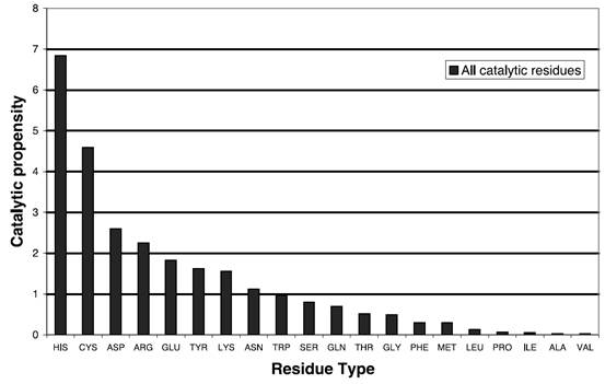
FIGURE. Catalytic propensity of different residues in enzymes determined by Janet Thornton et al (Bartlett, et al., 2002).

The score of residues submitted to PLS regression in FunSPRINT is directly obtained from the value of catalytic propensity in the above figure.

pKa changes (structure feature)

pK_a is a logarithimic acid dissociation constant (k_a) . Protonation states of ionizable residues can be determined by the environment pH values and pK_a values.A residue having pK_a shift can possibly serve as an active site (Ko, et al., 2005). The pK_a value is calculated from the package PROPKA (http://propka.ki.ku.dk/) (Li, et al., 2005).

Solvent accessibility surface area, or SASA (structure feature)

Solvent-accessible surface area (SASA) is an indicator of the accessibility of surrounding solvent to a molecule, acquired by tracing the locus of the center of a sphere with an approximately 1.4Å radius rolling over the van der Waals radii of atoms on the molecular surface of interest.

The SASA of residues were previously found to be an important feature of catalytic sites. Our statistics also find that higher percentage of catalytic residues than that of non-catalytic ones have relatively low SASA, shown in the Figure below. We use the package NACCESS to calculate the relative SASA (RSA) for each residue in the protein (Lee, et al., 1971; Hubbard, et al., 1993).

Distance to mass center of protein domains (structure feature)

According to the Figure below, we first decide whether the protein contains one or two domains by examining the mass distributions of proteins on their biggest principal components (see the Figure below). If two Gaussian distributions fit the histogram better than one Gaussian, we then consider the protein have two domains; otherwise, it has only one domain. Residues’ distances to their closest mass center (if it is a two-Gaussian distribution) are determined as one of the features for PLS regression.

(a) (b)

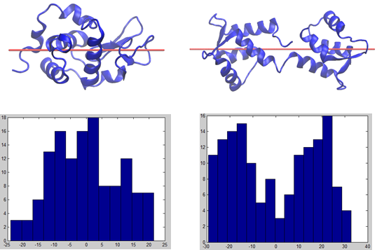
FIGURE. Residues projection on the largest principle component of the protein mass distribution. (a) and (b) are the Hen egg white lysozyme and Calmodulin structures, respectively. Red axes are the largest principal components (1^st PCs) to illustrate the widest variance of protein mass distributions. (c) and (d) are the histograms of projections of residues in (a) and (b) onto their corresponding 1^st PC axes with a unit of Å. ‘0’ means the mass centers of the proteins.

* Weighted clustering scores (structure feature)

After the first PLS giving scores, the top ranked hinge groups will be given a clustering score to reflect how close they are to other hinge groups. The score actually is weighted according to whether they are nearest to the top two ranked (heavily weighted), 3rd-7^th ranked, or 8^th-20th ranked hinge groups (minimally weighted). Thornton’s Thornton’s early work (Bartlett, et al., 2002) demonstrated that the clustering of top-ranked residues, suggested by an artificial neural network model, does help the prediction substantially.

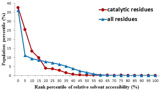
* Deviation of RSA of neighboring residues (structure feature)

After the first PLS regression, we measure the difference between the Relative Solvent Accessible Surface Area (RSA) of a residue and that of its secondary neighbors in the primary sequence. Our statistics (the Figure below) show that the different distributions between catalytic and non-catalytic residues, where 0% ranking in the horizontal axis indicates the largest RSA difference and 100% is the smallest.

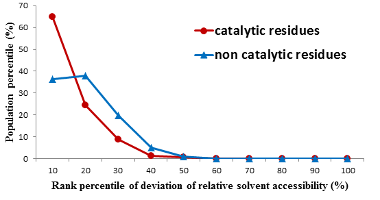
FIGURE. Residues distribution per their relative ranking of the RSA differences between themselves and their second neighbors

Dynamics hinges (dynamics feature)

A hinge group is composed of a consecutive 5 residues with the central residue having the smallest vibration magnitude among the five, where vibration magnitude of residues is defined by the superimposition of the three normal modes obtained from GNM (only hinge centers below 10% of the highest fluctuation in a molecule are considered). The global hinge centers predicted by the GNM were found to be co-localized with the catalytic sites experimentally identified (Yang, et al., 2005).

About PLS regression -

Compare to the traditional multiple regression analysis, the PLS is not limited by any assumption on the distribution of the raw data (Fornell et al., 1982), and require relatively few samples. Even the variables with moderate correlations can be handled successively. As for normal multiple regression analysis, the input variables must be normally distributed which is not true in our case. Therefore, we chose to use the PLS regression to build the prediction model.

Suppose existingindependent variables , dependent variables and samples, we can express the data by independent and dependent variables in matrix form and , respectively.

(1)

(2)

Before the PLS, we standardize the raw data by

(3)

(4)

where and indicate the element of the i-th row and j-th column of the independent matrix and dependent matrix, respectively. and terms for the average value over the j-th column the independent matrix and dependent matrix, respectively. and terms for the standard deviation of the j-th column the independent matrix and dependent matrix, respectively. The standardized matrices are denoted as

(5)

(6)

Suppose are the basis of dependent matrix, which can be represented as

, (7)

where are the weighting of each principle component, and is the projection on the first principle component. The basis can be extracted by decomposing the variance matrix comprising independent and dependent variables , which can give the unit eigenvector corresponding to the maximal eigenvalue. We then obtain

, (8)

where is the projection of the independent variables on its first principle component, also called the latent variable which serves as the basis of regression.

Further, by decomposing the variance matrix , we obtain the unit eigenvector corresponding to maximal eigenvalue. We then obtain

, (9)

where is the projection of the dependent variables on their first principle component. For the first principle components and of independent and dependent variables, respectively, there are two restrictions: first, and should be the best principle components to express the independent and dependent terms, respectively. Second, and should correlate strongly. With this, the extraction of the first principle component is done.

Then, we can substitute the first component for the regression formula of the independent variable matrix as follow:

, (10)

where are the weighting of each principle components for the regression formula of independent matrix, and is the weighting of the first principle component.

In the same way, we substitute the first principle component for the regression formula of the dependent variable matrix as follow, where is the weighting of the first principle component of the dependent variable matrix.

and that are the residues after the contribution of the first principal component is subtracted from and . 及 can be expressed as:

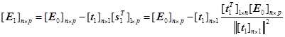(11)

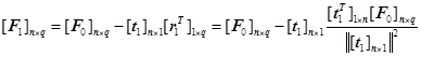(12)

Consequently, we can extract the second principle component from the residue variance matrix of the independent and dependent variables. Therefore, we can repeat the method extracting stated above to extract other principle components. The iteration algorithm is given as follow:

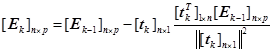
If we want to extract the k-th principle component,

(13)

(14)

(15)

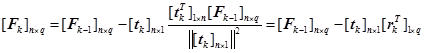(16)

where , ). In the study, we will extract all of the principle components to build the regression equation, hope to achieve the best PLS regression effect.

Reference

Bartlett GJ, Porter CT, Borkakoti N, Thornton JM. (2002). Analysis of catalytic residues in enzyme active sites. J. Mol. Biol. 15;324(1):105-21

B. Lee and F. M. Richards. (1971). The interpretation of protein structures: estimation of static accessibility. J. Mol. Biol. 55, 379-400.

Fornell C., Bookstein F. (1982). Two structural equation models: LISREL and PLS applied to consumer exit-voice theory. Journal of Marketing Research, 19(4), 440-452.

Glaser, F., Pupko, T., Paz, I., Bell, R.E., Bechor-Shental, D., Martz, E. and Ben-Tal, N. (2003).ConSurf: identification of functional regions in proteins by surface-mapping of phylogenetic information.Bioinformatics, 19, 163-164.

Hubbard,S.J. and Thornton,J.M. (1993)‘NACCESS’Computer Program. Department of Biochemistry and Molecular Biology, University College London.

Ko, J., Murga, L.F., André, P., Yang, H., Ondrechen, M.J., Williams, R.J., Agunwamba, A., and Budil, D.E. (2005). Statistical criteria for the identification of protein active sites using Theoretical Microscopic Titration Curves. Proteins 59, 183–195.

Li, H., Robertson, A.D., and Jensen, J.H. (2005). Very fast empirical prediction and rationalization of protein pKa values. Proteins 61, 704–721.

Yang, L.-W., and Bahar, I. (2005). Coupling between catalytic site and collective dynamics: a requirement for mechanochemical activity of enzymes. Structure 13, 893–904.